Any intervention by the government distorts the market. In most cases, a distortion favours one market participant over another. For example, when the government decides to invest in building a port, it favors traders and developers over other tax payers. Thus it disturbs the market process and eventually leads to inefficient allocation of resources. This is the logic used by Monetarists (those who advocate monetary policy as a tool for economic management) to oppose fiscal measures to counter business cycles.
The same logic used to oppose fiscal measures can in fact be extended to quantitative easing (QE) as well. QE distorts the most important of the markets: the market for money. QE to the uninitiated is the central bank buying securities (mostly government bonds) with the hope that the money will support the economy. There are two severe problems with this: Firstly, money does not create goods and services. It is only an enabler. So any dole out in the form of direct benefit or by purchasing assets is a redistribution of wealth. Secondly, any intervention by the government will directly benefit those who receive the money first. Any trickle down to others in the market is secondary. This creates an inequality. Any manipulation of money supply will help those who own assets (especially bonds) and puts at disadvantage those who do not have those assets but are looking to buy assets in future. Thus, banks, asset managers, wealthy individuals with investments, etc., benefit at the cost of salaried employees who want to acquire a house and other assets in the future after accumulating enough savings.
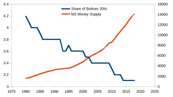
The graph below shows the trend of total money supply of US$(M2: i.e. including bank checking deposits) and the share of income of bottom 20% of US. As the money supply has been increasing overtime since 1980s, the share of the poor in income is decreasing. The income share of bottom 20% of Americans has come down from 4.2% in 1980 to 3.1% in 2018. There could be other metrics of income inequality as well but this one is easy to understand and track.
 The relationship is expressed strongly through the equation:
Income share of bottom 20% = -0.48 x log(M2) + 7.63
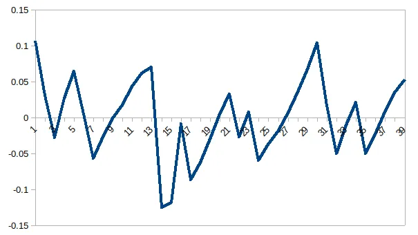
Such strong relationships can be spurious most of the times as both the variables (money supply and income inequality) have been trending in one direction, or to use fancy language they are non-stationary. To check if the relationship is not spurious we observe the residual (i.e. errors) of the above equation. As a shown below, the residual is stationary (i.e. it is not trending in one direction).
 This relationship where two variables are closely tied to each other is called co-integration. This gives credence to the theory that income inequality and money supply are closely related (at least in the US from 1980–2020). It can be argued that the relationship might be running the other way round, i.e. increasing income inequality is driving money supply up. But the data suggests that any deviation in the relationship causes income inequality to adjust and not money supply (to keep the article pithy I’m not posting the causal relationship analysis here). Which proves that money supply drives income inequality and not vice versa. Of course, there is the caveat that the data is especially on income inequality is sparse. Nevertheless, the data analysis strengthens the economic logic above.
Lastly I want to add that all income inequality is not necessarily bad. If the income inequality is accompanied by increase in incomes of both the poor and the wealthy, it may be on the whole beneficial to the poor. But having a more equitable growth will help the poor much more than just a top line income/GDP growth number. Misplaced priorities of some central banks could be a hindrance to this.
This relationship where two variables are closely tied to each other is called co-integration. This gives credence to the theory that income inequality and money supply are closely related (at least in the US from 1980–2020). It can be argued that the relationship might be running the other way round, i.e. increasing income inequality is driving money supply up. But the data suggests that any deviation in the relationship causes income inequality to adjust and not money supply (to keep the article pithy I’m not posting the causal relationship analysis here). Which proves that money supply drives income inequality and not vice versa. Of course, there is the caveat that the data is especially on income inequality is sparse. Nevertheless, the data analysis strengthens the economic logic above.
Lastly I want to add that all income inequality is not necessarily bad. If the income inequality is accompanied by increase in incomes of both the poor and the wealthy, it may be on the whole beneficial to the poor. But having a more equitable growth will help the poor much more than just a top line income/GDP growth number. Misplaced priorities of some central banks could be a hindrance to this.